轮腿机器人二自由度闭式连杆机构正逆运动学推导

1. 问题背景

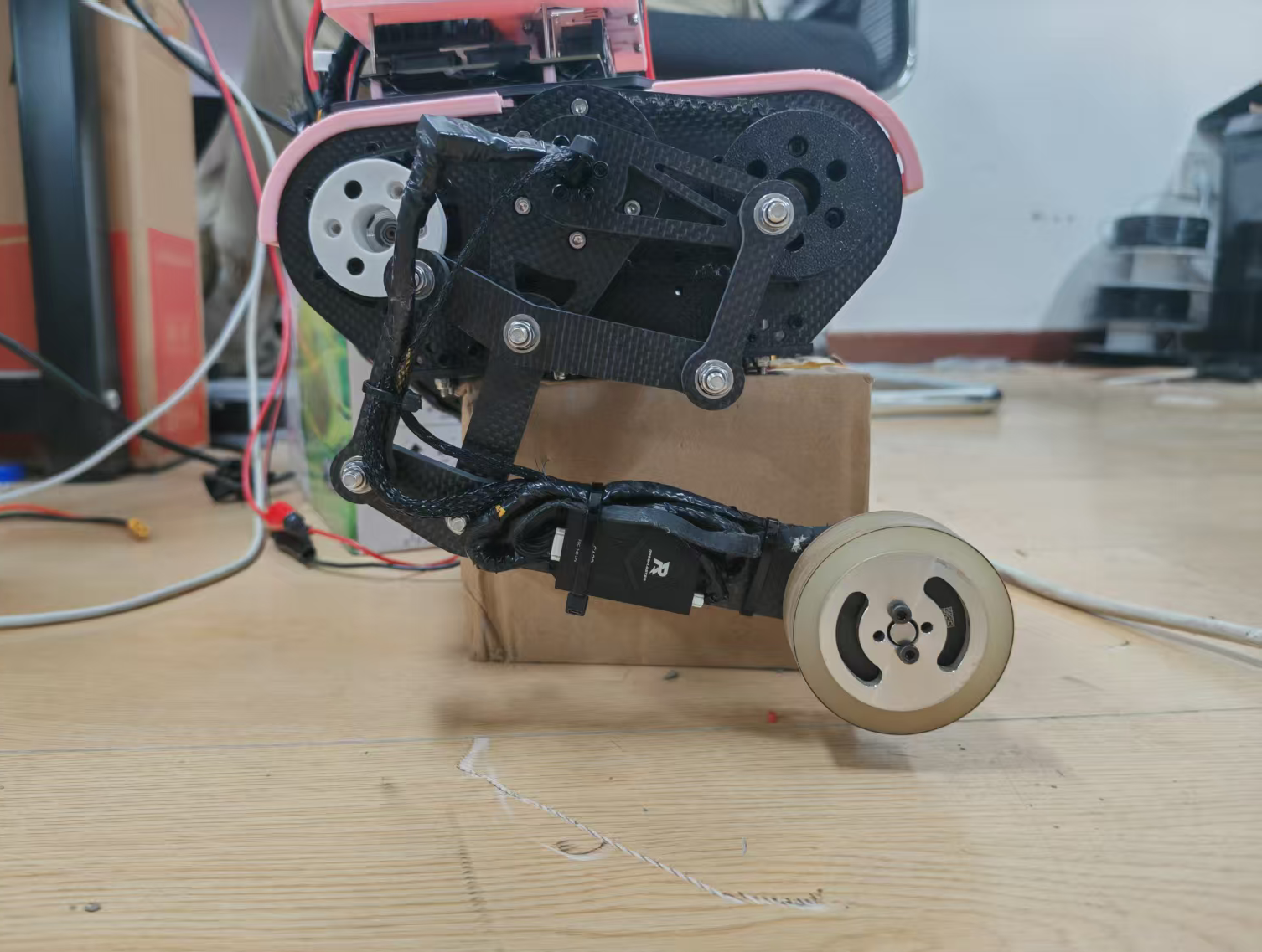
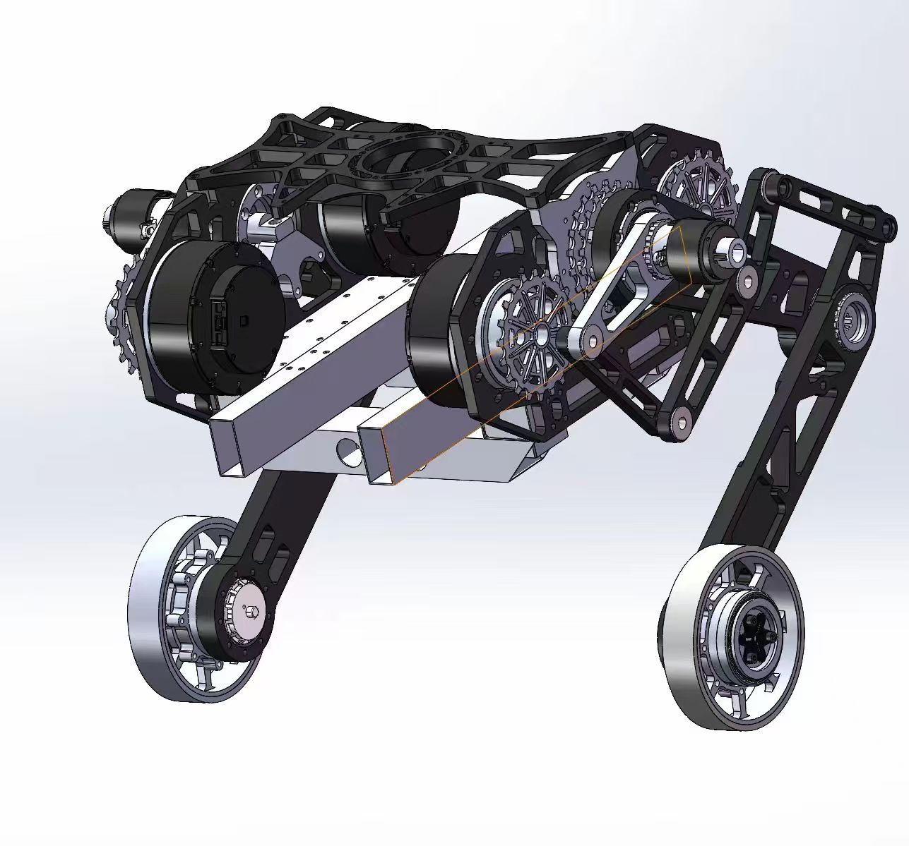
轮腿式机器人（wheel-legged robot）的每条腿需要同时具备 轮式滚动 和 腿部越障 两种能力。本文讨论的机构设计采用两个同轴电机，通过一套 8 字形双平行四边形连杆将动力传递到轮端，实现腿部摆动与轮子转向的解耦控制。

与传统带传动或齿轮传动方案相比，这种全连杆机构具有 零回程差、结构刚度高、无磨损件 等优点，特别适合需要高精度末端位置控制的轮腿机器人应用。

flowchart TD
  M["电机 A (θa)"] --> A["bar_a（三副杆 O-P1-P2）"]
  M2["电机 B (θb)"] --> B["bar_b（二副杆 O-P3）"]
  A --> D["bar_d（三副直杆 P1-P4-P5）"]
  B --> C["bar_c（二副杆 P3-P4）"]
  C --> D
  D --> E["bar_e（二副杆 P5-P6）"]
  A --> F["bar_f（三副直杆 P2-P6-P7）"]
  E --> F
  F --> W["P7 — 轮毂电机（末端）"]

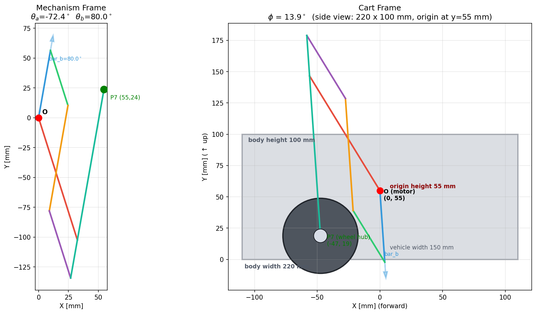
两个平行四边形嵌套成 8 字形：

• 平行四边形 1：O – P1 – P4 – P3，边长 48.4 × 57.3 mm
• 平行四边形 2：P1 – P2 – P6 – P5，边长 59 × 32.4 mm

2. 正运动学推导

正运动学的目标是：给定电机转角 $\theta_a, \theta_b$，求末端 $P_7$ 的位置。

2.1 点坐标逐步求解

Step 1 — bar_a 上的 P1、P2

以 O 为原点，绕 $\theta_a$ 旋转：

$$\begin{aligned} P_1 &= L_{OP1} \begin{bmatrix}\cos\theta_a \\ \sin\theta_a\end{bmatrix} = 48.4 \begin{bmatrix}\cos\theta_a \\ \sin\theta_a\end{bmatrix} \\[6pt] P_2 &= L_{OP2} \begin{bmatrix}\cos\theta_a \\ \sin\theta_a\end{bmatrix} = 107.4 \begin{bmatrix}\cos\theta_a \\ \sin\theta_a\end{bmatrix} \end{aligned}$$

这里 $L_{OP2} = 48.4 + 59 = 107.4$，因为 bar_a 是直杆，P1 在 O–P2 连线上。

Step 2 — bar_b 上的 P3

$$P_3 = L_b \begin{bmatrix}\cos\theta_b \\ \sin\theta_b\end{bmatrix} = 57.3 \begin{bmatrix}\cos\theta_b \\ \sin\theta_b\end{bmatrix}$$

Step 3 — bar_d 上的 P4（两圆相交）

由平行四边形 1 可知 $|P_1P_4|$、$|P_3P_4|$ 为固定值，故 P4 是两圆的交点：

• 圆心 $P_1$，半径 $L_{P1P4} = 57.3$
• 圆心 $P_3$，半径 $L_c = 48.4$

两圆相交的解析求解过程如下。令向量 $\mathbf{v} = P_3 - P_1$，两圆心距离 $d = \|\mathbf{v}\|$，则：

$$\begin{aligned} a &= \frac{L_{P1P4}^2 - L_c^2 + d^2}{2d} \\[4pt] h &= \sqrt{L_{P1P4}^2 - a^2} \\[4pt] P_4 &= P_1 + \frac{a}{d}\mathbf{v} \pm \frac{h}{d}\mathbf{R}\mathbf{v} \end{aligned}$$

其中 $\mathbf{R} = \begin{bmatrix}0 & -1 \\ 1 & 0\end{bmatrix}$ 为 $90^\circ$ 旋转矩阵，$\pm$ 号的选择对应两种装配模式，记作 $\mathrm{branch}\_d = \pm 1$。

2.2 核心简化：直杆约束

得到 P4 后，bar_d 的方向角为：

$$\theta_d = \text{atan2}(P_4 - P_1)$$

因为 bar_d 是 直杆，P5 与 P1、P4 共线，且 $|P_1P_5| = 32.4$，所以：

$$P_5 = P_1 + \frac{32.4}{57.3} (P_4 - P_1)$$

代入平行四边形 2 的关系 $P_6 = P_2 + P_5 - P_1$，消去 P5：

$$P_6 = P_2 - \frac{32.4}{57.3} (P_4 - P_1)$$

注意 $P_4 - P_1$ 的方向与 $P_3$ 相同（平行四边形对边平行），而 $P_3 = L_b[\cos\theta_b, \sin\theta_b]^T$，于是：

$$P_6 = P_2 - 32.4 \begin{bmatrix}\cos\theta_b \\ \sin\theta_b\end{bmatrix}$$

bar_f 同样是直杆，P7 在 P2→P6 的反方向延长线上，$|P_2P_7| = 128$：

$$P_7 = P_2 + 128 \begin{bmatrix}\cos\theta_b \\ \sin\theta_b\end{bmatrix}$$

2.3 最终解析式

将 $P_2 = 107.4[\cos\theta_a, \sin\theta_a]^T$ 代入，得：

$$\boxed{P_7 = \begin{bmatrix} 107.4\cos\theta_a + 128\cos\theta_b \\ 107.4\sin\theta_a + 128\sin\theta_b \end{bmatrix}}$$

infographic list-grid-badge-card
data
  title 物理意义
  desc 机构等价于一个标准 2R 平面机械臂
  items
    - label 第一连杆
      desc O → P₂，长 L₁ = 107.4 mm，角度 θa
      icon mdi/link-variant
    - label 第二连杆
      desc P₂ → P₇，长 L₂ = 128 mm，角度 θb
      icon mdi/link-variant
    - label 末端
      desc 轮毂电机位置 P₇
      icon mdi/wheel

3. 逆运动学推导

逆运动学：给定末端位置 $P_7 = (x, y)$，求 $\theta_a, \theta_b$。

3.1 余弦定理

令 $r = \sqrt{x^2 + y^2}$（P7 到原点的距离），$\phi = \text{atan2}(y, x)$。

由 2R 机械臂的几何关系：

$$\cos\alpha = \frac{r^2 + L_1^2 - L_2^2}{2 L_1 r}$$ $$\alpha = \arccos\left(\frac{r^2 + 107.4^2 - 128^2}{2 \times 107.4 \times r}\right)$$

3.2 两个解

$$\theta_a = \phi \pm \alpha$$

正号对应 elbow-down，负号对应 elbow-up（两种臂型）。

$$\theta_b = \text{atan2}\left( y - L_1\sin\theta_a,\; x - L_1\cos\theta_a \right)$$

3.3 工作空间与奇异位形

工作空间是一个圆环：

$$|L_1 - L_2| \leq r \leq L_1 + L_2$$

即 $20.6 \text{ mm} \leq r \leq 235.4 \text{ mm}$。

三种奇异位形：

条件	含义	解的情况
$r = L_1 + L_2 = 235.4$	完全伸展	单解（$\theta_a = \theta_b$）
$r = \|L_1 - L_2\| = 20.6$	完全收缩	单解
$r = 0$	末端与原点重合	无穷多解

在奇异位形附近，机构的传力性能会急剧下降——微小的末端力就可能在关节处产生很大的力矩。这也是 2R 机械臂的固有问题，在轨迹规划时需要避开奇异区域。

4. 代码实现

4.1 两圆相交

这是整个数值求解的几何基础——给定两个圆心和半径，求交点。

def circle_intersection(c1, r1, c2, r2):
    """返回 (p_left, p_right)，无解时返回 (None, None)。"""
    v = c2 - c1
    d = np.linalg.norm(v)

    if d < 1e-12:          # 同心圆
        return None, None
    if d > r1 + r2 + 1e-10 or d < abs(r1 - r2) - 1e-10:
        return None, None  # 无交点

    a = (r1**2 - r2**2 + d**2) / (2.0 * d)
    h = np.sqrt(max(r1**2 - a**2, 0.0))
    p_mid = c1 + (a / d) * v

    if h < 1e-10:
        return p_mid.copy(), p_mid.copy()  # 相切

    perp = np.array([-v[1], v[0]]) / d
    return p_mid + h * perp, p_mid - h * perp

通过 perp 向量的正负号区分两个解——对应两种装配模式。

4.2 正运动学求解器

def solve_linkage(theta_a, theta_b, params, prev_theta_d=None, prev_theta_f=None):
    # 1. bar_a 上的 P1, P2
    P1 = rotate_vec(np.array([params.L_OP1, 0.0]), theta_a)
    P2 = rotate_vec(params._a2_local, theta_a)

    # 2. bar_b 上的 P3
    P3 = params.L_b * np.array([np.cos(theta_b), np.sin(theta_b)])

    # 3. 两圆相交求 P4
    p4_left, p4_right = circle_intersection(P1, params.L_P1P4, P3, params.L_c)
    # prev_theta_d 用于轨迹跟踪时保持分支连续性

    # 4. bar_d 方向 → P5
    theta_d = np.arctan2((P4 - P1)[1], (P4 - P1)[0])
    P5 = P1 + rotate_vec(params._d5_local, theta_d)

    # 5. 两圆相交求 P6
    p6_left, p6_right = circle_intersection(P2, params.L_P2P6, P5, params.L_e)

    # 6. bar_f 方向 → P7（末端）
    theta_f = np.arctan2((P6 - P2)[1], (P6 - P2)[0])
    P7 = P2 + rotate_vec(params._f7_local, theta_f)

    return {'P7': P7, 'theta_d': theta_d, 'theta_f': theta_f, ...}

整个求解过程全部由三角函数和开方完成，无需任何迭代，属于纯解析正解。

4.3 逆运动学

def solve_inverse(P7_target, params, elbow=1):
    L1, L2 = params.L_OP2, params.L_P2P7
    x, y = P7_target
    r = np.hypot(x, y)

    if r > L1 + L2 + 1e-6 or r < abs(L1 - L2) - 1e-6:
        return []  # 超出工作空间

    cos_alpha = (r**2 + L1**2 - L2**2) / (2.0 * L1 * r)
    alpha = np.arccos(np.clip(cos_alpha, -1.0, 1.0))
    phi = np.arctan2(y, x)

    solutions = []
    for sgn in ([-1, 1] if elbow == 0 else [elbow]):
        theta_a = phi + sgn * alpha
        theta_b = np.arctan2(
            y - L1 * np.sin(theta_a),
            x - L1 * np.cos(theta_a),
        )
        solutions.append({'theta_a': theta_a, 'theta_b': theta_b})

    return solutions

5. 四种装配模式

两圆相交的 $\pm$ 选择带来了 四种装配模式（branch_d × branch_f），对应实际机构的不同组装方式：

infographic list-grid-badge-card
data
  title 四种装配模式
  desc 两圆相交 ± 解的组合 → 四种装配模式
  items
    - label "凸凸 (−1, −1)"
      desc P₄ 在 P₁→P₃ 左侧，P₆ 在 P₂→P₅ 左侧
    - label "凸凹 (−1, +1)"
      desc P₄ 在 P₁→P₃ 左侧，P₆ 在 P₂→P₅ 右侧
    - label "凹凸 (+1, −1)"
      desc P₄ 在 P₁→P₃ 右侧，P₆ 在 P₂→P₅ 左侧（★ 默认模式）
    - label "凹凹 (+1, +1)"
      desc P₄ 在 P₁→P₃ 右侧，P₆ 在 P₂→P₅ 右侧

其中 $\mathrm{branch}\_d = +1,\ \mathrm{branch}\_f = -1$（凹凸）对应两个平行四边形均为凸四边形的情况，这也是 2R 简化成立的默认模式。

其余三种模式中平行四边形会出现不同程度的凹陷，但正逆运动学的解析推导框架仍然相同——仅在求解时选择对应的 $\pm$ 分支即可。不过需要注意，非默认模式下的末端 P₇ 与电机轴的相对方位会发生变化，在轨迹规划时应与默认模式区分对待。

5.1 轨迹跟踪中的分支保持

轨迹跟踪时，每一帧的 solve_linkage 会传入上一帧的 $\theta_d, \theta_f$，在两圆相交的两个解中选取与上一帧更接近的那个。这样就能在连续运动中保持同一装配模式，避免跳跃。

# 选取与上一帧更接近的 P4（保持 branch_d 连续性）
P4 = p4_left if norm(p4_left - P4_prev) <= norm(p4_right - P4_prev) else p4_right

同理，P6 的分支选择也采用相同的近邻判定策略。完整的分支保持逻辑如下：

def select_branch(p_left, p_right, p_prev):
    """从两个交点中选取与上一帧更接近的那个"""
    if p_prev is None:
        return p_left  # 首帧，默认取第一个
    d_left = norm(p_left - p_prev)
    d_right = norm(p_right - p_prev)
    return p_left if d_left <= d_right else p_right

这两个分支选择算法共同保证了轨迹跟踪过程中两个平行四边形都能保持连续的装配状态，不会出现"跳帧"导致的运动不连续或机构卡死。

5.2 装配模式的选择依据

默认模式（凹凸, +1, −1）是物理装配最自然的方案——两个平行四边形均保持外凸，机构受力状态最佳，且与 2R 简化模型直接对应，便于运动学规划。

在某些特殊运动需求下（如需要避开障碍物、改变末端姿态范围或优化传力角度），可以选择其他装配模式。装配模式的切换需要在机构经过奇异位形（两圆相切，$h = 0$）时自然过渡——此时两个解重合，分支可以安全切换。

6. 验证

$\theta_a$	$\theta_b$	$P_7$（解析）	$P_7$（数值）
0°	90°	(107.4, 128.0)	(107.4, 128.0) ✓
30°	120°	(29.0, 164.6)	(29.0, 164.6) ✓
0°	0°	(235.4, 0.0)	(235.4, 0.0) ✓
−30°	45°	(183.5, 36.8)	(183.5, 36.8) ✓

以上验证表明，解析推导与数值求解完全一致，正逆运动学求解器正确可靠。

7. 总结

这套 8 字形双平行四边形机构巧妙地利用了 直杆共线 约束，使得看似复杂的连杆传动链最终简化为一个 2R 平面机械臂。正逆运动学均有闭式解析解，无需数值迭代，非常适合嵌入式实时控制场景。

如果你对完整代码感兴趣，项目在 GitHub 上开源：

# 快速体验
git clone https://github.com/729DHS/linkage-2dof.git
cd linkage-2dof
uv sync
python main.py interactive   # 交互式滑块
python main.py anim          # 生成动画
python main.py ik            # 逆运动学演示

---